Course Notes for VE406 (Applied Regression Analysis using R) | FA2020 @UM-SJTU JI, Shanghai Jiao Tong University.

This is the markdown(.md) version note. Another note with R code (.Rmd version) is available here, and pdf version is also included.

Linear regression

Based on l08

1. datasize 是否小datasize无法用central limit theorem

2. descriptive analysis: look at the data

3. explorative analysis: density plot of all variables

   binomal for independent variable: two

4. scatterplot matrix: to see the relationship between dependent and independent variables, which may violate the assumption that (x are independent)
   lattice::splom

5. shapiro-wilk test: for small data size: check normality (not y|x, but x)

6. F-test between models

7. with the chosen model: do diagnotics

8. Cook distance: the influential points

9. detect multicollinearity: variance inflation factor (VIF)

attention points

• lack of data: small data set leads to no strong evidence available
• do not use t-test to select variables
• select model: compare the full model with the submodel (adj. R squared)
• claim the purpose: to explain or to predict
• to determine whether a polynomial term is needed: plot standardised residual against each of the regressor
• only drop variables after checking the assumption
• The SE of the sample slope, the value under SE Coef. Again, the SE of any statistic is a measure of its accuracy. In this case, the SE of b1 gives, very roughly, the average difference between the sample b1b1and the true population slope β1β1, for random samples of this size (and with these x-values).
• shapiro.test: <0.1 -> not normal

1. $R^2$: a measure of goodness of fit when all assumptions are satisfied

   however, larger value of $R^2$ do not indicate:

   • assumptions are satisfied
   • better predictive model
   • better model across all data set
   • better model when models have different number of parameters

2. adjusted $R^2$: relative measure to address: when models have different number of parameters

   • Can not be interpreted alone
   • can not used for two models that have different response

confused point

Cook’s distance

L08 L10

• outliers: extreme response values $y_i|x_i$, possible large $\hat{e}_i$, 应该看vertical distance to the regression line

• leverage point: points with extreme $x_{ij}-values$ relative to others, (may not have large residuals)， 所以不一定为outlier，看的是横向的是否x与其他的点偏离

  

  但这并不一定不好，如果该数据样本与得到的预测模型相符合时，（利比亚对其周边国家）这个样本即可进行核实和加强。但差别较大（利比亚与发达国家）时，会使其偏离真实模型。

  所以要比较移除/保留leverage point会造成怎样的影响，是否要进行transformation

• influential point : a point whose deletion would significantly alter the regression surface.

  • Quantification methods:

    1. Standardized difference in coefficients

       
    2. 

    3. Cook’s distance: based on the idea of confidence ellipsoid

• Cook's distance：Cook’s D measures how much the model coefficient estimates would change if an observation were to be removed from the data set. higher cook’s D, higher influnce.

  Generally accepted rules of thumb are that Cook’s D values above 1.0 indicate influential values, and any values that stick out from the rest might also be influential.

  意义依然是将原模型得到的预测值和移除第个样本后的预测值进行比较，从调参经验中我们将设置阈值设为，高于阈值的数据样本需要移除。

interaction

L08

The interaction term has this meaning or interpretation: consider the relationship between Y and Z. So far in this course, this relationship has been measured by b , the regression coefficient of Y on Z. This coefficient Z is a partial coefficient in that it measures the impact of Z on Y when other variables have been held constant. But suppose the effect of Z on Y depends on the level of another variable, say X. Then, bZ by itself would not be enough to describe the relationship because there is no simple relationship between Y and Z. It depends on the level of X. This is the idea of interaction.

So a interaction variable by multiplying, W = XZ. Then add the term into model

• add the interaction term, based on the t-test p_value determine whether the interation term is significant
• visualize through interaction plot

stability problem

L10

from the $Var[\hat{\beta_1}]$, it has two parts, and the accuracy of our model is determined by

• the amout of scatter about the true regression line, measured by $\sigma$,
• “configuration” of observed $x_i$, that is, the spread of the observed $x_i$

Analyze the configuration

1. With one predictor
   • spread out $x_i$ -> well supported regression line, little change under resampling.
   • bunched up $x_i$ -> unstable regression line, like a seesaw

2. two predictor $X_1$ and $X_2$

   the spread and correlation are both important

   • strong relationship -> tends to have a “knife edge”
   • uncorrelated/orthogonal -> spread out, support the fitted plane

3. in general

   

Multicollinearity occurs when the column of the data matrix are almost linearly dependent

https://statisticsbyjim.com/regression/multicollinearity-in-regression-analysis/

• happens when

  1. One or more predictors have very little variation (this predictor almost constant compared to others can’t explain variation in y)
  2. One or more predictors have vey large mean (they should have same scale leave residuals small)
  3. Two or more predictors have a linear relationship

  The frist two (inessential) could be removed by standardising the data

  The last one (essential) could not be reduced by standardising.

• How to detect multicollinearity?

  1. general method: looking at the standard error of slope,

  2. through variation inflation model (VIF): 1: no correlation, 1-5:moderate correlatoin, >5: critical

Heteroskedasticity

constant variance is violated

do not care about fit model but care about prediction, this problem could be ignored. because it

studentized residuals

A studentized residual is calculated by dividing the residual by an estimate of its standard deviation. The standard deviation for each residual is computed with the observation excluded. For this reason, studentized residuals are sometimes referred to as externally studentized residuals.

With weighted least squares, it is crucial that we use studentized residuals to evaluate the aptness of the model, since these take into account the weights that are used to model the changing variance. The usual residuals don't do this and will maintain the same non-constant variance pattern no matter what weights have been used in the analysis.

VIF

variance inflation factor: This is a measure of how much the standard error of the estimate of the coefficient is inflated due to multicollinearity.

1.0: no collinearity: orthogonal

5-10: might problematic

$>10$ : severe. when VIF=100, this would mean that the other predictors explain 99% of the variation in the given predictor.

auxiliary response

When do weighted least squares, to determine the appropriate weights

https://online.stat.psu.edu/stat501/lesson/13/13.1

• Store the residuals and the fitted values from the ordinary least squares (OLS) regression.
• Calculate the absolute values of the OLS residuals. $[z=2*(log(abs(lm\$residuals)))]\rightarrow auxiliary \ response$
• Regress the absolute values of the OLS residuals versus the OLS fitted values and store the fitted values from this regression.$[auxiliary \ regression]$ These fitted values are estimates of the error standard deviations.
• Calculate weights equal to $1/fits^2$, where "$fits$" are the fitted values from the regression in the last step.

We then refit the original regression model but using these weights this time in a weighted least squares (WLS) regression.

Log transformation

From midterm exam

• Why do we need to do log transformation for the response $y$?

  1. Reduce the variance in $y$
  2. after log transformation (if have interaction for different variables), the trend of different parameters might change (one might have more increasing rate after transformation). Without log transformation, the judge might be wrong

• What’s the impact of log transformation?

  \begin{align*} y&=\beta x \\ log(y)& = \beta x\\ \end{align*}

  Then, when say holding every other variables constant, increase x by 1 unit will cause y to increase between $lowerboundof\hat{\beta}$ and $upperboundof\hat{\beta}$ will no longer be correct.

  We need to do the ratio to know how much it will changed after log transformation.

  \begin{align*} log(y_1) - log(y_2) &=\hat{\beta}(x_1-x_2) = log\left(\frac{y_1}{y_2}\right) \\ \frac{y_1}{y_2} &=exp(\hat{\beta}(x_1-x_2)) \end{align*}

  So the exp of the difference gives us not the increase, but the multiply relationship.

  This will be really important for the nonlinear regression and the regression introduced afterwards.

Non-linear regression

**Always remember inference might not be appropriate for small data size **

Always remember back transformation!

Bootstrapping

The bootstrap is a technique in statistics which consists of resampling the observed data in order to create an empirical distribution of some statistic

how to answer the question such that (confidence interval of model parameter / how to describe the uncertainty around the fitted values of the model / )

1. Let $r$ denote the number of bootstrap replications—that is, the number of bootstrap samples to be selected
2. For each bootstrap sample b = 1,... ,r, randomly draw n observations with replacement from among the n sample values, and calculate the bootstrap sample mean,.
3. From the r bootstrap samples, estimate the standard deviation of the bootstrap means

• 在训练集里有放回的重采样等长的数据形成新的数据集并计算相关参数，重复n次得到对参数的估计，计算标准误差
• 生成Bootstrap Percentile置信区间
• 适用于独立样本，样本间有相关如时间序列数据可采用block法分组屏蔽掉进行bootstrap
• 因为存在重复，使用bootstrap建立训练集与预测集会有非独立样本，造成检验集模型方差的低估，去掉重复使模型复杂，不如交叉检验对检验集误差估计的准 （cite https://yufree.github.io/notes/section-11.html)

see also: https://www.math.pku.edu.cn/teachers/lidf/docs/statcomp/html/_statcompbook/sim-bootstrap.html

mosaicplot

display categorical data

Example:

Interpretation:

• more survival in 1st class, more female & child survive
• …

Odds and Odds ratio

Odds: describe the ratio of success to ratio of failure.

simple example

Gender \ Purchase	Yes	No
Female	106	159
Male	125	121

Female group: $Odds=\frac{106/(106+159)}{159/(106+159)}=1.5$

Higher the odds, better is the chance for success. Odds will be in $[0,+\infty]$.

Odds Ratio: the ratio of odds. will be in $[0,+\infty]$.

represents which group has better odds of success.

Odds Ratio for females = Odds of successful purchase by female / Odds of successful purchase by male = $\frac{106/159}{121/125}$

Logistic Regression

unlike previous continuous response

use logistic function

$\text{Pr}(Y=1|X=x)=m(x,\mathbf{\beta})=\frac{exp(\beta_0+\beta_1x)}{1+exp(\beta_0+\beta_1x)}$

odds

$o_S=\frac{p}{1-p}$

as modelling the response were binomially distributed as

$Y_i|X_i \sim Binomial(mean=prob=m_i,size=1) \\ mean: \mathbb{E}[Y|X]=m \quad variance:\text{Var}[Y|X]=m(1-m) \\ Group: S_i|X_i \sim Binomial(mean=prob=m_i,size=n_i)$

with the success probability depending on the regressors/predictors. The estimate is obtained through maximum likelihood function

• Transform from linear regression to logistic regression

? Logistic regression but not classification

​ In linear regression, $X$ and $Y$ ranges from $[-\infty,+\infty]$. $Y$ now categorical data (0 / 1). So predict probability $[0,1]$ instead of dinstinct value 0 / 1.

\begin{align*} Y&=a+b_iX_i, &-\infty\leq Y\leq \infty,\ &-\infty\leq X_i\leq \infty\\ P&=a+b_iX_i, &0\leq P\leq 1,\ &-\infty\leq X_i\leq \infty (Probability)\\ P/(1-P)&=Odds=a+b_iX_i, &0\leq Odds\leq \infty,\ &-\infty\leq X_i\leq \infty \\ log(Odds)&=a+b_iX_i, &-\infty\leq log(Odds)\leq \infty,\ &-\infty\leq X_i\leq \infty\\ \end{align*}

​ we have achieved a regression model, where the output is natural logarithm of the odds , also known as logit. The base of the logarithm is not important but taking logarithm of odds is.

​ Then the probability of success is

\begin{align*} Odds&=e^{a+b_iX_i}=\frac{P}{1-P};&P=\frac{1}{1+e^{-(a+b_iX_i)}} \\ \frac{\hat{P}}{1-\hat{P}}&=exp(\hat{\beta}x) &\hat{P}=\frac{exp(\hat{\beta}x)}{1+exp(\hat{\beta}x)} \\[2ex] log(\hat{Odds})&=\hat{\beta}x \\[4ex] &\text{how to find odds ratio}\\ log(\frac{P_1}{1-P_1})&=\beta x_1 & log(\frac{P_2}{1-P_2})&=\beta x_2 \\[1.5ex] log(\frac{P_1}{1-P_1})-&log(\frac{P_2}{1-P_2})=\beta (x_1-x_2) \\[1.5ex] odds \ ratio&= exp(\beta (x_1-x_2)) &\text{the odd of}\ x_1 \text{is} \ exp(\beta (x_1-x_2))\ \text{higher than } x_2 \end{align*}

• How to interpret coefficient

https://stats.idre.ucla.edu/other/mult-pkg/faq/general/faq-how-do-i-interpret-odds-ratios-in-logistic-regression/ For different types

1. Logistic regression with no predictor variables
2. Logistic regression with a single categorical binary (only 0/1) predictor variables
3. Logistic regression with a single continuous predictor variable
4. with multiple predictor variables and no interaction terms
   • estimated coefficient: change in the log odds of being in an honors class (type 1) for a unit increase in the corresponding predictor variable holding the other predictor variables constant at certain value.
   • exponential coefficient: odds ratio, or the change in odds in the multiplicative scale for a unit increase in the corresponding predictor variable holding other variables at certain value
5. with an interaction term of two predictor variables
   • attempts to describe how the effect of a predictor variable depends on the level/value of another predictor variable.
   • could not talk about the effect of one term while holding other terms as constant (because of the interaction term involving this term)

# to understand the odds ratio in logistic regression, analyze one output 

## 
## Call:
## glm(formula = admit ~ gre + gpa + rank, family = "binomial", 
##     data = mydata)
## 
## Deviance Residuals: 
##    Min      1Q  Median      3Q     Max  
## -1.627  -0.866  -0.639   1.149   2.079  
## 
## Coefficients:
##             Estimate Std. Error z value Pr(>|z|)    
## (Intercept) -3.98998    1.13995   -3.50  0.00047 ***
## gre          0.00226    0.00109    2.07  0.03847 *  
## gpa          0.80404    0.33182    2.42  0.01539 *  
## rank2       -0.67544    0.31649   -2.13  0.03283 *  
## rank3       -1.34020    0.34531   -3.88  0.00010 ***
## rank4       -1.55146    0.41783   -3.71  0.00020 ***
## ---
## Signif. codes:  0 '***' 0.001 '**' 0.01 '*' 0.05 '.' 0.1 ' ' 1
## 
## (Dispersion parameter for binomial family taken to be 1)
## 
##     Null deviance: 499.98  on 399  degrees of freedom
## Residual deviance: 458.52  on 394  degrees of freedom
## AIC: 470.5
## 
## Number of Fisher Scoring iterations: 4


# For every one unit change in gre, the log odds of admission (versus non-admission) increases by 0.002

exp(cbind(OR = coef(mylogit), confint(mylogit)))

##                 OR   2.5 % 97.5 %
## (Intercept) 0.0185 0.00189  0.167
## gre         1.0023 1.00014  1.004
## gpa         2.2345 1.17386  4.324
## rank2       0.5089 0.27229  0.945
## rank3       0.2618 0.13164  0.512
## rank4       0.2119 0.09072  0.471

#  for a one unit increase in gpa, the odds of being admitted to graduate school (versus not being admitted) increase by a factor of 2.23.

• The dependent variable in logistic regression follows Bernoulli distribution with unknown probability $P$.

Therefore, the logit i.e. log of odds, links the independent variables ($Xs$) to the Bernoulli distribution.

• likelihood ratio test: LR-test of significance / variable selection

  similar to F-test of significance and partial F test $H_0:$ the reduced model is sufficient

however, we donot have methods to check the validity of the model and the appropriateness of using the asymptotic approximation, care with small n!

• reduced model deviance

  test on $\beta_2 = 0$, reduced model do not have $\beta_2$, full model includes $\beta_2$, the deviance difference between these two models should have a chi-square distribution with $r$( number of $\beta_2$) degrees of freedom, reject with a large value. (in case that null hypothesis is true and $n$ is large).

• Test on individual model coefficients

  $H_0: \beta_j=0$ Wald statistic

glm with family=binomial in R.

1. non-grouped: outcome is provided as a vector of 0/1 or a factor with two levels, with the predictors on the rhs of your formula
2. grouped data: there are group of data points that have the same $\mathbf{X}$.
   • give a matrix with two columns of counts for success/failure as the lhs of the formula.
   • use the weights= argument to indicate how many positive and negative outcomes were observed for each category of the classification table.

? if we useingots.LG = glm(notready/total~heat+soak, family = binomial, data = ingots.df, weights = total), notready/total is probability, what’s weights for? why not regression

• For grouped data,

  1. diagnostics for linearity and independence can be done using Pearson residuals.

     However, for samll data size, will not be very informative in terms of linearity or independence, but for small data size pearson still can be used to identity outliers, high leverage points and influential points.

     

  2. the deviance of a model plays a similar role that RSS has a multiple linear regression (the larger the deviance, the worse the fit) (zero deviance means no information lost).

     the deviance $R^2$ for a model $A$ is defined as $R_d^2=1-\frac{d_A}{d_0}$, where $d_0$ is the deviance of the null model (such that the logistic regression only includes the intercept $m(\mathbf{X},\beta_0)=\frac{exp(\beta_0)}{1+exp(\beta_0)}$.

Poisson Regression

unlike previous two type (continous / binary response), response as count

each individual response

$Y_i|X_i \sim Poisson(mean=var=m_i)$

with mean depends on the regressors / predictors

• deviance test for poisson: scaled deviance

当响应变量观测的方差比依据泊松分布预测的方差大时，泊松回归可能发生过度离势，而且发生的概率很大。可能发生过度离势的原因有如下几个：

• 遗漏了某个重要的预测变量；
• 可能因为事件相关，在在泊松分布的观测中,计数中每次事件都被认为是独立发生的。
• 在纵向数据分析中，重复测量的数据由于内在群聚特性可导致过度离势。

Generalized Linear Model

relax some assumptions of MLR

need: independent $Y$ and errors

• Linear function, e.g. can have only a linear predictor in the systematic component
• Responses must be independent

Multiple linear regression is a regression with multiple independent variables. What makes the model linear is that there are coefficients on each variable (rather than nonlinear functions of each variable). There are many ways to estimate the value of these coefficients, the most common of which is ordinary least squares. Ordinary least squares (OLS) makes assumptions about the elements of the error term that are not always appropriate for every problem - that they are independent/incorrelated to each other.

Generalized least squares is a way to relax the assumption of independent errors. It begins by estimating the correlation between elements of the error term and using that correlation in a least squares model with more realistic assumptions.

In summary, linearity is about the functional form of the regression equation; generalizability is about the method to estimate coefficients. So they're not mutually exclusive - you can certainly run a generalized multiple regression.

need to know:

• exponential family of the underlying distribution
• the link function
• the linear predictor of the response variable to explotary variables

The choice of link is separate from the choice of random component thus we have more flexibility in modeling

https://online.stat.psu.edu/stat504/node/216/

GEE

quasi-likelihood estimate, parameter estimate is valid even when the covariance matrix is mis-specified.

https://online.stat.psu.edu/stat504/node/180/

specify the appropriate error distribution for the response and the implied link function, and an argument to specify the structure of the working correlation matrix (within-cluster correlation).

the independence is assumed between clusters

Non-parametric

Only need: linear predictor

The fitted values under a linear smoother is simply gievn by

$\hat{y_i}=\hat{m}(x_i) \Rightarrow \mathbf{\hat{y}=Sy}$

where matrix $\mathbf{S}$ is known as smoothing matrix

• a smoother curve does not mean better, especially for prediction, because less variance involved
• break the ordered data into segments, for each segment, fit the data with simple or kernel

Simple Smoothing

1. binning / bin-smoothing: will have discontinuous at the boundary
   • have a fixed-width bins with varying number of observations
2. simple moving average (SMA), often used in time-seires
   • $(n-L)$ bins, each has fixed number of observations
   • results a shift in $x$ for a large $L$ due to only using “past” data
3. simple central moving averages (SCMA)
   • $(n-2L)$ bins
   • avoids the shift in $x$ by using data on both sides
   • no estimated value of $m(x)$ at two endpoints of $x$
4. running mean smoothing (RMS)
5. running line smoothing (RLS)

the simple smoothers are not smooth, one way to address is to use a linear spline rather than a least squares line. Specifically, some called cubic spline. the coefficients are chosen at the observed data only. the result will rely on the data chosen

Kernel Smoothing / Regression

a kernel is a non-negative integrable function $K(z)$ such that

$K(z)=K(-z),\ \int_{-\infty}^{\infty}K(z)dz=1,\ \mathop{lim}_{z\rightarrow -\infty}K(z)= \mathop{lim}_{z\rightarrow \infty}K(z)=0$

common kernel functions: Rectangular / Triangular / Parabolic / Gaussian

• bandwidth $h$ $\hat{m}_h(x)$

Penalised Regression

• natural cubic interpolating spline (NCIS)

Spline Interpolating

样条插值，给出a set of data points, 要求连续且一阶导连续（曲线光滑），二阶导连续（曲线曲率最小），且二阶导在boundary point为0

Regression splines often give better results than polynomial regression. This is because, unlike polynomials, which must use a high degree polynomial to produce flexible fits, splines introduce flexibility by increasing the number of knots but keep the degree fixed.

Generalised Additive Model

it is a glm, more than one explotary variables. Like glm use unknown relations. Need a link funtion, relating y to the predictors, through smoothing funciton s

Non-identifiable model

additive model

check the error, which assume zero mean and constant variance

The main difference imho is that glm assume a fixed linear or some other parametric form of the relationship between the dependent variable and the covariates, GAM do not assume a priori any specific form of this relationship, and can be used to reveal and estimate non-linear effects of the covariate on the dependent variable.

Pearson residuals for GLM and GAM should have approximately zero mean and constant variance

PCA

https://zhuanlan.zhihu.com/p/26305845

主要判断准则如下：

1. 根据先验经验和理论知识判断主成分数；
2. 根据要解释变量方差的积累值的阈值来判断需要的主成分数；
3. 通过检查变量间k×k的相关系数矩阵来判断保留的主成分数。

• Difference in PCA and FA

  PCA: a method, FA: an application

  Simplistically, though, factor analysis derives a mathematical model from which factors are estimated, whereas PCA merely decomposes the original data into a set of linear variates

• Factor Rotation:

  factor loading：大部分variables会对most important factor 有high factor loading，但不方便interpretation

  Factor rotation used to discriminate between factors. A factor is a classification axis along which variables could be plotted, factor rotation effectively rotate these factor axes such that variables are loaded maximally on only one factor.

  旋转是一系列将成分载荷阵变得更容易解释的数学方法，其作用是尽可能地去除噪声。旋转可以分为正交旋转和斜交旋转，前者使选择的成分保持不相关，后者让它们相关。

Factor Analysis

When assume there is some hidden structure from which the observed $\mathbf{X}$ are generated, may need other dimension reduction method.

• factor model used to model such hidden structure: The variability in a large number of observed variables could be due to few unobserved factors and unobserved errors

  $\mathbf{X}_{n\times k}=\mathbf{F}_{n\times k}\mathbf{W}^k_{k\times l} + \mathbf{\epsilon}_{n \times k}$

  $l < k \rightarrow $ Dimension reduction

  • **manifest variables: ** $\mathbf{X}$ , which is observed, as the original definition
  • **latent factors: **$\mathbf{F}$, hidden variables

  Specification:

  • $\mathbf{X,F}$ : zero mean + unit variance

  • $\mathbf{\epsilon:}$ zero mean

  • $\mathbf{F}$ uncorrelated across observations and with other latent factors

  • $\mathbf{\epsilon}$ uncorrelated across observations, across $\mathbf{X} \text{ and }\mathbf{F}$

Some Points

• not nested model, can;t use deviance based test, likelihood test, to select model

  • could use AIC, the smaller, the better

• Use deviance to check goodness of fit. Use scaled deviance for GAM

  

Summary

Models and Assumption check:

写出用了什么模型，得到了什么结果，check 了什么assumption，因此又fit了什么，最终得到的model是什么

Executive Summary

想要test什么，得到了什么结论，estimate结果

要review的问题：

• 为什么要用各个模型
• 各个模型背后的assumption是否有什么特定的，如何check，assumption violate了怎么办
• 如何interpret estimate of each model
• gamma response with inverse / log link

GLM:

need: independent $Y$ and errors

• Linear function, e.g. can have only a linear predictor in the systematic component (non-parametric / GAM当不再linear)
• Responses must be independent (GEE 解决这一条的violation: solve the correlation error non-parametrically || GLMM through a probability model)

GLM要求response independence当有repeated response observations violate independence 于是有了GEE

nonparametric 与 nonlinear不同：modelling only one independent variable + form of $m(x)$ not being assumed or given beforehand. including : smoothing , linear spline instead of least square line. ONLY NEED linear predictor

GAM do not assume a priori any specific form of this relationship, and can be used to reveal and estimate non-linear effects of the covariate on the dependent variable. The main difference imho is that glm assume a fixed linear or some other parametric form of the relationship between the dependent variable and the covariates,

PCA and FA 是用于polish the exploratory variables

• SLR is a special case of MLR, MLR is a special case of GLM, GLM is a special of GAM

• everything is a trade-off, heavier computitional power for loose condition

LR test

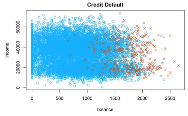
credit.all3.LG = glm(default~balance+income+student, family = binomial, data = credit.df)
summary(credit.all3.LG) 
# LR test of significance, similar to F-test
credit.null.LG = glm(default~1, family = binomial, data = credit.df)
LR.test = 2*(logLik(credit.all3.LG)[1] -logLik(credit.null.LG)[1]) 
# compare full with null model, so three beta reduced to zero, degree of freedom should be 3 
1-pchisq(LR.test, 3) 
# significantly strong evidence to reject that the reduced model is adequate

# LR test for reduced, similar to partial F-test
credit.no.income.LG = glm(default~.-income, family = binomial, data=credit.df) 
# must be the submodel (to the model going to be compared)
LR.test = 2*(logLik(credit.all3.LG)[1] -logLik(credit.no.income.LG)[1])

1-pchisq(LR.test, 1) 
# fail to reject, only reduce one model, degree of freedom is 1 

# LR-test 
1-pchisq(bomber.PS$deviance,bomber.PS$df.residual)
# 0.46: large p-value -> no evidence of lack of fit 

# significance 
1-pchisq(bomber.PS$null.deviance,bomber.PS$df.null) 
# 0.0033: small p-value: at least one of the regressors is needed 

# GAM  use scaled deviance to check goodness of fit 

$R^2$ through deviance

# R_d^2 is 
1-sim.final.LG$deviance/sim.final.LG$null.deviance
# =0.97, model capture most of the deviation in the date