Xinmiao

Notes for VE477 (Introduction to Algorithms) | FA2020 @UM-SJTU JI, Shanghai Jiao Tong University.

Computational Problem

a computational problem is a question or a set of questions that a computer might be able to solve. (what is a computer?)
study of the solutions to the computational problem composes the field of Algorithms
computational complexity attempts to classify the algorithm depending on their speed or memory usage.

decision problem
search problem
counting problem
optimization problem
function problem

Turing Machine

a function $f: \sum^* \rightarrow \sum^*$ is said to be Turing computable if there exists a Turing machine $M$ which returns $f(x)$ for any input $x$ .

deterministic polynomial algorithm: $T_M(x)\leq P(x)$
$L$ a language, $P$ decision problem $P$

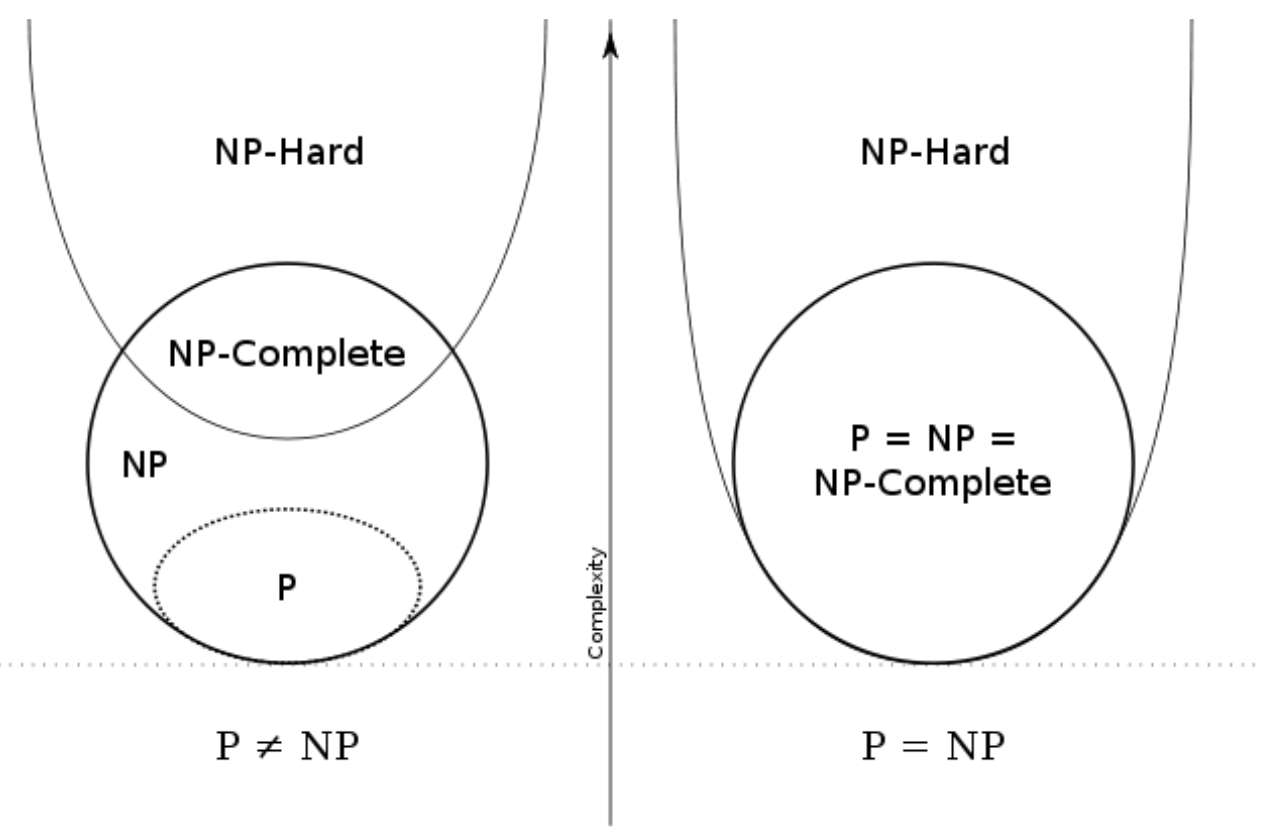
The set of the decision problems which could be solved by a deterministic polynomial algorithm defines the class P.

class NP: a decision problem is computable by a non-deterministic polynomial algorithm.
- be polynomial with the certificate
class co-NP
NP-Complete: NP-Complete is a complexity class which represents the set of all problems X in NP for which it is possible to reduce any other NP problem Y to X in polynomial time.
NP-hard: do not have to be in NP, do not have to be decision problem. a problem X is NP-hard, if there is an NP-complete problem Y, such that Y is reducible to X in polynomial time.

P问题是在多项式时间内可以被解决的问题，而NP问题是在多项式时间内可以被验证其正确性的问题。 NP困难问题是计算复杂性理论中最重要的复杂性类之一。如果所有NP问题都可以多项式时间归约到某个问题，则称该问题为NP困难。

$NP$ contains all problems in $P$

PSPACE completeness

SPACE: denote the set of all the decision problems which can be solved by a Turing machien in $\mathcal{O}(s(n))$ space for some function $s$ of the input size $n$ . PSPACE is defined as
$PSPACE = \cup_{k} SPACE(n^k)$
PSPACE-complete: 1. in PSPACE 2. for all $P$ in PSPACE, $P$ can be reduced in polynomial space the to $PSPACE-complete$

halting problem: undecidable. Do not belong to $NP$ . $NP-hard$ . reduce SAT to Halting problem

SAT

boolean satisfiability problem: NP-complete
TQBF: PSPACE-complete and NP-hard

True Quantiffied Boolean Formula: can be solved in exponential time and polynomial space.
- when quantifier $\forall$ , the both $x_i=0or1$ should be evaluted true
- $\exists$ , only one of them
Then each time recursive call will give at most 2 way, then $\mathcal{O}(n^2)$
Hilbert’s tenth problem

Given a Diophantine equation, with any number of unkown quantities and with rational integral numerical coefficients, decide whether the equation is solvable in rational numbers (decision problem).
3-SAT

example of how to proceed to evaluate the complexity class of a given problem

cnf: conjunctive normal form: if a boolean formula is written as the conjunction of disjunctive clauses.

3-SAT is NP-complete:
- 3-SAT is in $NP$ (clearly as it is a particular case of SAT)
- in $NP-complete$ that being able to solve it means being able to solve SAT, the proposed transformation is applicable in polynomial time
  
  Convert a cnf-formula $F$ to a 3cnf-formula $F’$ (then could transform any instance of SAT into an instance of 3-SAT)
  
  Denote each clause in $F$ as $C_1, C_2, ...,C_k$
  a. For clause has one literal as $x_1$ , change to $(x_1\lor x_1 \lor x_1)$
  b. For clause has two literals as $(x_1\lor x_2)$ , change to $(x_1\lor x_2 \lor x_1)$
  c. For clause has more than three literals as $(x_1\lor x_2\lor ... \lor x_m)$ , introduce new variable $z_i$ change to $(x_1\lor x_2 \lor z_1)\land (\neg z_1\lor x_3 \lor z_2)\land (\neg z_2\lor x_4 \lor z_3)\land ... \land (\neg z_{m-3}\lor x_{m-1} \lor x_m)$
  
  an example:
  
  Then we could rewrite it as
  
  $$
  \begin{align*}
  &(x_1\lor x_2 \lor z_1)\land (\neg z_1\lor \neg x_3 \lor z_2)\land (\neg z_2\lor x_4 \lor z_3)\land (\neg z_3\lor x_5 \lor\neg x_6)\land \
  &(\neg x_1\lor \neg x_2 \lor z_1)\land (\neg z_1\lor x_3 \lor z_2)\land (\neg z_2\lor\neg x_4 \lor z_3)\land (\neg z_3\lor x_5 \lor x_6)\land \
  &( x_1\lor \neg x_2 \lor z_1)\land (\neg z_1\lor \neg x_3 \lor z_2)\land (\neg z_2\lor x_4 \lor z_3)\land (\neg z_3\lor x_5 \lor \neg x_6)\land \
  &(x_1 \lor \neg x_2 \lor x_1)
  \end{align*}

stirling’s formula $n! \approx \sqrt{2\pi n}(\frac{n}{e} )^n$
$logn! \in \Theta(n \cdot logn), \lceil logn\rceil \in \Theta(logn)$

1+2+4+8+…+2^{log n} $\approx$ 2n-1. Thus, the time complexity is $\Theta(n)$ .

Running time is expressed as T(n) for some function T on input size n.

$T(n)\in O(f(n))$ also $T(n)= O(f(n))$

complexity theory

RAM model

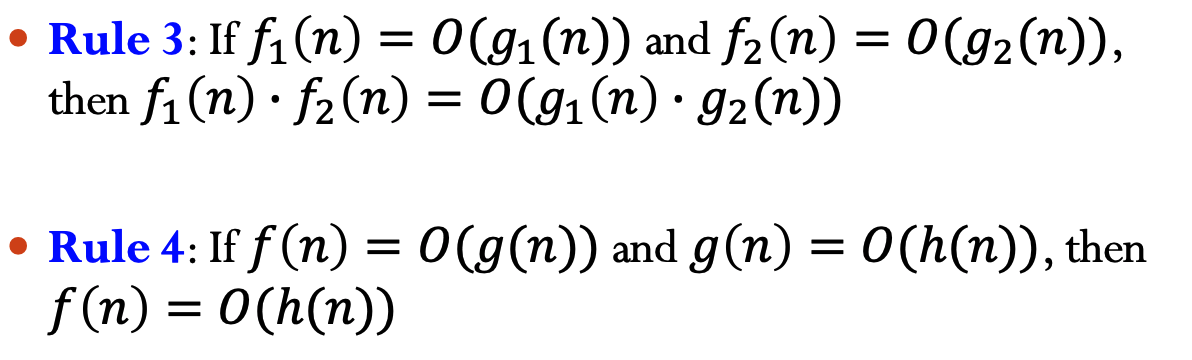
The complexity of an algorithm is defined by a numerical function

$\mathcal{O}$

A sufficient condition of Big-Oh

？

$\Omega$

$\Theta$

Solve Recurrence

Master method: $T(n) \leq aT(\frac{n}{b}) + O(n^d)$

base case: for sufficiently small $n$ , $T(n) \leq constant$
a = number of recursive calls (positive integer)
b = input size shrinking factor (positive integer)
$O(n^d)$ : the runtime of merging solutions. d is a real value $\geq $ 0
a, b, d : independent of n
1. In merge sort, a=2, b=2, d=1
2. in quick sort, if choose the median as the pivot, a=2,b=2,d=1
3. in binary search, a=1, b=2, d=0

Divide-and-conquer Approach

merge sort
Quick sort

Counting inversions

divide into 2 sets
in each set, recursively count the number of inversions
sort each sort
when merge, as need to compre the number, could get the number

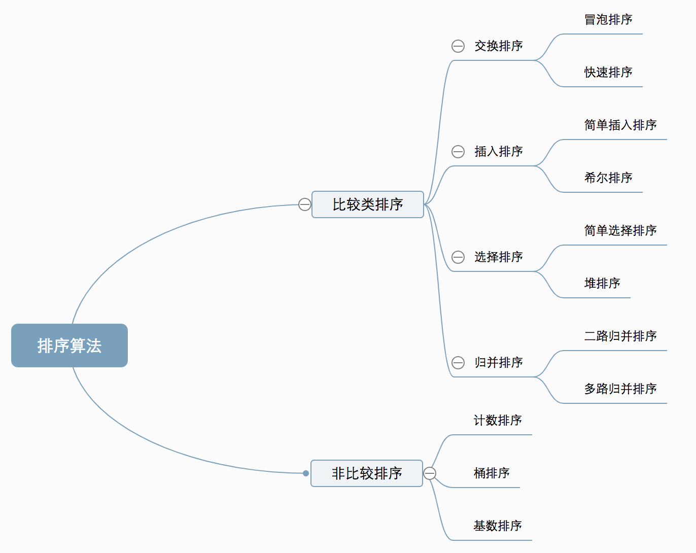
Sorting

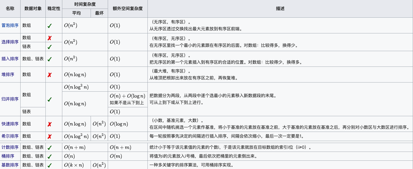
A sorting algorithm that is based on pairwise comparisons mush use $\Omega (NlogN)$ operations to sort in the worst case

Reorder array A of size N with consistent comparison function

in place: requires $\mathcal{O}(1)$ additional memory；不占用额外内存，只利用原来存储待排数据的存储空间进行比较和交换。

“ Space usage affects the constant factor, because the memory access takes time. Modern computers are based on memory hierarchy. The top is small cache, but extremely fast. If O(1) additional space, it can be fit inside the cache and then, the program is fast; otherwise, it cannot be fit inside the cache, which needs to read the secondary memory, which takes time. ”
Stability: whether the algorithm maintains the relative order of records with equal keys

	Best Case Time	Worst Case Time	Average Case Time	In Place	Stable
Insertion	O(N) sorted array	O( $N^2$ ) 逆序array	O( $N^2$ )	Yes	Yes
Selection	О(n2) comparisons, O(1) Swap	O( $N^2$ )	O( $N^2$ )	Yes	No
Bubble		O( $N^2$ )	O( $N^2$ )	Yes	Yes
Merge Sort		O( $N log⁡N$ )	O( $N log⁡N$ )	No	Yes
Quick Sort		O( $N^2$ )	O( $N log⁡N$ )	Weakly	No

Comparison Sort

Each item is compared against others to determine its order

Simple sorts

insertion sort
selection sort
bubble sort

Fast sort: quick sort and merge

Quick Sort

select a pivot randomly

worst case $\mathcal{O}(n^2)$ : 每次都选到了最大/最小的元素

出现可能 $\frac{2^{n-1}}{n!}$ - extremely samll

On average $\mathbb{\theta}(n)$

how to do partition? Not in place: with another array B

in-place partition

1. once select a pivot, swap the pivot with the first element in the array 
2. set two pointer i,j; i points to the second element in the array, i = 1; j points to the last elemtn j = N - 1
3. Then increment i until find A[i] >= pivot
4. decrease j until find A[j] < pivot
5. if i < j : swap A[i] and A[j] the go back to 3.  
6. otherwise swap the first element (the pivot) with A[j]

Non-comparison Sort / distribution-based sort

each item is put into predifined “bins”, independent of other items; no comparison with other items needed
Counting sort / bucket sort / radix sort

Counting sort

Assume that the input consists of data in a small range

给定array，已知其中data range为（0，k） + length of the array $A$ N (k and N are both parameters, although known, not treated as constant)

allocate a new array $count$ with size k+1
store the number of each number in the original array $A$ in $count$
Sum all number from $0$ to $k$ in $count$ as $count[i] = count[i] + count[i-1]$
from the end of $A$ , put each element in $A[n]$ in the new array at the position $count[A[n]]$ , then $count[A[n]] -=1 $

Bucket sort

Assume that the input is drawn from a uniform distribution, then linear time complexity $\mathcal{O}(n)$ could be obtained. (the time complecity is relevant to the input)

set an array as an initially empty bucket
Go over the array, put each item into corresponding bucket
in each bucket, do comparison sort
visit all the buckets in order and put all items back to the original array

Radix sort

比如sort name, 因为姓氏的集中性，not good for it

each element in the n-element array $A$ has $d$ digits, where digit 1 is the lowest-order digit and digit $d$ is the highest order.

In-place and not in-place both merge sort each subarray recursively, the difference is in the merge function. For the marge sort discussed in the class, $$\leq $$ is used to compare so that it is stable.

In-place merge sort need to shift all the element because no additional memory (like the additional array in slides), so time complexity $$O(n^2)$$ not $$O(nlogn)$$ any more.

LinearTime Selection

Randomized selection algorithm

Average :

Input array size n && random pivot choice

Rselect is in phase j: current array size is between $(\frac{3}{4})^{j+1}n$ and $(\frac{3}{4})^{j}n$ .

$X_j$ : the number of recursive calls in phase $j$

For example, phase 0 is size between [3/4n, n]. Depends on what the pivot you choose, the array may enter a new phase or remain in the current phase

Good pivot: make the left sub-array size is am, i.e. 1\4<a<3\4. Probability: 0.5. 因为只要在old array中间50%的位置取即可获得

E[ $X_j$ ]≤ Expected number of times you need to get a good pivot, p=0.5, == flip coin

小于：因为即使无good pivot也可能进入new phase

N: the number of chosen needed to get a good pivot. P[N=k] = $\frac{1}{2^k}$ ; E[N]=2.

E[ $X_j$ ] <= E[N] = 2

第一层循环中将pivot与n个元素进行比较，时间为 $cn$ .: 第一步时间 $T(n)=cn+T(n/2)$

相似的，在递归过程中 $T(n/2)=c(n/2) + T(n/4); \ T(n/4)=c(n/4) + T(n/8)…\ T(2) = 2*c+T(1); \ T(1)=1*c$

则有 $T(n) = c(n+n/2+n/4+…+2+1) = 2n = O(n)$

空间复杂度：无额外的空间，inplace $\mathcal{O}(1)$

The runtime depends on the input pivot

When i = n/2 ,the worst case runtime is $\mathcal{\Theta}(n^2)$ , such that example array 1,2,3,4,5,6,7, choose pivot sequence 1,2,3,7,6,5,4 then comparison time: c(n-1 + n-2 + … + n/2 + … 1). However, if choose 1,2,3,4,5,6,7, only c(n-1 + n-2 + … + n/2 )

Best:

Best case happens when your random selection of pivot directly gives you the i-th smallest item (i.e., a pivot with index as i). However, the pivot index can only be known after the partition. Thus, the runtime is $\mathcal{\Theta}(n)$ .

Deterministic selection algorithm

Idea: use “median of medians”

ChoosePivot(A, n)

A subroutine called by the deterministic selection algorithm
Steps

1.Break A into n/5 groups of size 5 each

2.Sort each group (e.g., use insertion sort)

3.Copy n/5 medians into new array C

4.Recursively compute median of C

By calling the deterministic selection algorithm!

5.Return the median of C as pivot

Dselect

Intpu array size n; Runs on $\mathcal{O}(n)$ time

but not in-place: need an additional array of 5/n medians

对于长度为5的array排序，时间为constant，
why size <= 0.7n

于是可以看出在图中T(?)处的size不会大于0.7n

因此对于整个dselect来说，

Hope: there is a constant a (independent of n) such that T(n)≤an for all n>1

Then T(n)=O(n)

We choose a=10c, so to prove ->

Proof by induction:

base case: $T(1) \leq 10c$
inductive step: inductive hypothesis $T(k) \leq 10ck, \forall\ k<n$

Then prove it also true for $T(n)$ : $T(n) \leq cn+T(\frac{5}{n}) + T(\frac{7n}{10}) \leq cn+2cn+7cn = 10cn$

Dynamic Programming

idea behind DP:

break a complex problem into simpler subproblems
store the result of the overlapping subproblems
do not recompute the same information again and again
do not waste memory because of recursion

saves both time and space

simple idea dramatically improving space-time complexity
cover all the possibilities at the subproblem level
efficient as long as the number of subproblems remains polynomial

eg: fibnonacci number naive way: do recursion

Memorized DP: recursion + memorization

**time = #of sub problems $\cdot$ time/subproblem **

mem={}
fib(n):
	if n in mem: return mem[n]
	else:
		if n <= 2: f = 1
		else: f = fib(n-1) + fib(n-2)
		mem[n] = f
		return f
// # of subproblem:n & time/subproblem is \Theta(1)

fib(k) only recurses when it is first called
only n nonmemorized calls: k=n, n-1, … 1
memorized call free ( $\Theta(1)$ time)
could ignore recursion, $\Theta(1)$ time per call

https://www.zhihu.com/question/23995189

Bottom-up DP

fib = {}
for k in [1,2, ...,n]: # n loops, each call is \Theta(1)
		if k <= 2: f = 1
		else: f = fib(n-1) + fib(n-2)
		fib[k] = f
return fib[n]
// same computation as do not need to count for recursion but save space

intro

用尽量少的1，5，11凑出15；贪心策略 $15 = 1 * 11 + 4 *1$ , 五张。

正确的为 $15 = 3 * 5$ ，三张。贪心策略为尽量使之后面对的w更少，只考虑眼前情况

用 $f(n)$ 表示凑出n所需要的最少数量。与1，5，11各用了多少无关。

Cost = f(4) + 11 / f(10) + 5 / f(14) + 1 -> $f(n) = min{ f(n-1),f(n-5),f(n-11)} + 1 $

以 $\mathcal{O}(n)$ 复杂度解决

将一个问题拆成几个子问题，分别求解这些子问题，即可推断出大问题的解
Definitions: (DP 需要满足的前提)
- 无后效性：确定f(n)后，如何凑出f(n)即无关
- 最优子结构: f(n)即为小问题的最优解，因此可以得出大问题的最优解
DP: 枚举有可能成为答案的解，自带剪枝 - 尽量缩小可能解空间

knapsack problem

subset sum problem

time complexity $\mathcal{O}(N*sum)$

Use a boolean subset[i][j] to denote if there is a subset of sum j with element at index $i-1$ as the last element.

subset size: (A.size() + 1) * (target + 1)
subset[i][j] = True
## sum of a subset with the i-1 th element as the last element, equal to j

if (A[i] > j)
	subset[i][j] = subset[i - 1][j]  // copy the answer for previous cases
else 
	subset[i][j] = subset[i - 1][j] OR subset[i - 1][sum - A[i]]
	// if any previous states have already experinced the sum=j OR 
	// OR any previous state experinced a value 'j - A[i]'

Shortest path

Implementation: dij & bellmanford in VE477 lab5 (lab4: fib heap)

shortest path in weighted graph: Given a connected, simple, weighted graph, and two vertices $s$ and $t$ , find the shortest path that joins $s$ to $t$ .

Egdes only have positive weights
Edges have positive and negative egdes

Dijkastrs’s algorithm: only for solving the case 1, could not deal with negative weights. (no DP involved)
Bellman-Ford: take advantage of DP

Subproblem dependency should be acyclic

String

when subproblem for strings: (all polynomial)

Suffixes $x[i:], \forall i$ $\Theta(n)$
prefixes $x[:i,], \forall i$ $\Theta(n)$
substrings $x[i:j], \forall\ i\leq j$ $\Theta(n^2)$

Edit Distance:

given two string $x$ and $y$ , the cheapest possible sequence of character edits to turn $x\rightarrow y$ .

ALLOW:
- Insert $c$
- Delete $c$
- replace $c$ with $c'$
SUBPROBLEM: $x[i:]\&y[j:]\ \forall i,j$ then $\Theta(|x|\cdot|y|)$

GUESS: one of three allowed possibilities

RECURRENCE: DP(i, j) = min{ (cost of repalce x[i]->y[j] + DP(i+1, j+1) , cost of insert y[j] + DP(i, j+1), cost of delete x[i] + DP(i+1, j)}

TOPO ORDER: i: |x| -> 0

j: |y| ->0

DP( $\emptyset, \O$ )

Time comlexity: subproblem $\Theta(1)$ . Total: $\Theta(|x|\cdot|y|)$

longest common sequence: $HELLO$ for these two words

$x: HIEROGLYPHOLOGY$

$y: MICHAELANGELO$

Union-Find

A disjoint-set data structure is a data structure that keeps track of a set of elements partitioned into a number of disjoint (non-overlapping) subsets. A union-find algorithm is an algorithm that performs two useful operations on such a data structure:

并查集是一种树型的数据结构，用于处理一些不交集的合并及查询问题; 不能将在同一组的元素拆开

two operations

Find(v): find the root of the tree for vertex $v$
Union(v, w): link the root of the tree containg vertex $v$ to the root of tree containing vertex $w$

两处优化

When Find, update all the nodes along the path (all link them to the root directly)
When Union, set the root with higher depth as the parent of another root (minimize the depth of the tree)

Complexity

Lemma
iterated logarithm function

such that, the iterated algorithm of n is the number of time that the function log need to be applied to obtain a number smaller than 2
The cost for one find operation is $\mathcal{O}(logn)$

because for each find, the path will be compressed,
The amortized time for a sequence of $m$ GenSet Union Find operations, $n$ of which are GenSet can be performed in time $\mathcal{O}(m\alpha(n))$ .

The complexity of Union-Find structure is $\Omega(\alpha(n))$

Ackerman’s function

inverse Ackerman’s function

MST

Implement: VE477 lab2 (Minimum Spnning Tree)

Definitions

tree: acyclic, connected undirected graph; $|E| = |V| - 1$
any connected graph with $N$ nodes and $N-1$ edges is a tree
graph $G=(V,E)$ , subgraph $G’ = (V’,E’)$ iff $V’\subseteq V \& U’\subseteq U$
spanning tree of a connected undirected graph $G$ is a subgraph of $G$ that contains all the nodes and is a tree.
weighted, connected and undirected graph -> MST, which is a spanning tree with the minimum sum of weights.
$T$ is a tree: if it contained a cycle, at least one edge could be removed, allowing a lower weight while preserving the connected property of $T$

Algorithms

a. Prim’s Algorithm
- $V = T \cup T’$ , $T:$ nodes added to MST; $T’:$ nodes not in MST
- For each node $v \in T’$ , keep a measure $D(v)$ storing current smallest weight over all edges that connect $v$ to a node in $T$
- Keep $P(v)$ for each node $v$ : $(P(v), v)$ is the edge chosen in MST
Full version:
1. Pick one node $s$ , set $D(s) = 0$ , for any other node $v$ , set $D(v)=\infty$ and $P(v)$ unknown
2. Set $T’ = V$
3. While $T’ \neq \emptyset $
- For all nodes in $T’$ , choose a node $v$ that has the smallest $D(v)$ .
- Remove $v$ from set $T'$
- For $v’s$ neighbors $u$ that still in $T’$ , if exist $D(u)>w(v,u)$ , then update $D(u)$ as $w(v,u)$ and $P(u)$ as $v$
b. Kruskal’s Algorithm

Greedy Algorithm, union-find data structure
- sort all the edges $G.E$ by weight
- for edges in $G.E$ in non-decreasing order, adding them into $T$ if no cycle would be created
To check whether a cycle will be created, union find: whether two edges have the same root Find ; add them: Union

Network flow

网络流问题

对flow的限制：容量限制和流量守恒
Antiparallel: $(v_1,v_2)\in E \ and \ (v_2,v_1)\in E$
multiple source and/or sink nodes: super node

Maximum Network Flow Problem

Residual graph $G_f$ . ( $|E_f|\leq 2|E|$ ) 残存图
Argumenting path 增广路径. Residual capacity: on an argumenting path $p$ , the maximum flow that could be added to each edge s. 将沿着增广路径重复增加路径上的流量直到找到一个最大流. How to know we find a maximum flow? A flow is the maximum flow if and only if no argumenting path in the residual networks.
cuts of flow networks: One cut $(S,T)$ of flow network $G=(V,E)$ , cut the $V$ as $S \ and\ \ T=V-S, s\in S,t\in T$ .

If $f$ is a flow, then the net flow $f(S,T)$ across the cut $(S, T)$ is defined to be

$f(S,T)=\sum_{u\in S}\sum_{v \in T} f(u,v) - \sum_{u\in S}\sum_{v \in T} f(v,u)$

The capacity of a cut $S(S,T)$ is: $c(S,T)=\sum_{u\in S}\sum_{v \in T} c(u,v)$ .
Minimum cut: A minimum cut of a network is a cut whose capacity is minimum over all cuts of the network.

Max-flow Min-cun Theorem

Algo. Examples

counting inversions

of low implement: VE477 lab3.1.1

数逆序对 application: voting theory / analysis of search engines ranking / collaborative filtering

Divide and conquer approach 将list分为两半，recursively sort list并记录count (sort and count). 接着将两个list (merge and count)

Algorithm. (Merge and count)
Input : Two sorted lists: L1 = (l1,1,··· ,l1,n1), L2 = (l2,1,··· ,l2,n2) 
OutpuT: Number of inversions count, and L1 and L2 merged into L
Function MergeCount(L1 , L2 ):
  count ← 0; L ← ∅; i ← 1; j ← 1; 
  while i≤n1 andj≤n2 do
  	if l1,i ≤ l2,j then
  		append l1,i to L; i++;
  	else
  		append l2,j to L; count←count + n1 − i + 1; j++; end if
  end while
  if i > n1 then append l2,j,··· ,l2,n2 to L; 
  else append l1,i,··· ,l1,n1 to counL;
  return count and L
end

Algorithm. (Sort and count)
Input : A list L = (l1,··· ,ln)
Output : The number of inversions count and L sorted

Function SortCount(L):
  if n=1 then return 0 and L; 
  else
  	Split L into L1 = (l1,··· ,l⌈n/2⌉) and L2 = (l⌈n/2⌉+1,··· ,ln); 
  	count1, L1 ← SortCount(L1);
  	count2, L2 ← SortCount(L2);
  	count, L ←MergeCount(L1, L2);
  end if
  count ← count1 + count2 + count;
  return count and L 
end

time complexity: For merge O(n)

sort part: every time spilt it into two equal parts, a=2, b=2, f(n) = O(n), $T(n) = \Theta(n^{log_ba}logn) = \mathcal{O}(nlogn)$

So total for Sort and Count is $\mathcal{O}(n \rm{log} n)$

Stable Marriage Problem

Algorithm: Gale-Shapley

Implements 477 Lab3.1.2

Time complexity $\mathcal{O}(n^2)$

N Queens Puzzle

Implementation: Leetcode #52

8*8棋盘上，皇后可以横直斜走，格数不限。皇后之间不可以相互攻击->任何两个皇后不可以在同一行，同一列以及同一斜线上。

backtracking:

Data Structure

A bit comparison of different data structure.

Array has better memory locality and cache performance, arrays are contiguous memory blocks, so large chunks of them will be loaded into the cache upon first access.

	Dictionary
	Array (Unsorted/Sorted)
`search(D,k)`
`insert(D,k)`
`delete(D,k)`
`predecessor(D,k)`
`successor(D,k)`
`minimum(D)`
`maximum(D)`

Dictionary using array

Dictionary using linked structure

Hashing

Basics

Setup: a universe $U$ of objects (eg. all names, .., very big)
Goal: maintain an evovling set $S\subseteq U$ (eg. 100 names, … ,reasonable size)
original solution: array based / linked list based

Better solution

Hash table, an array A of n buckets $n=c|S|$
hashing function $h: U \rightarrow {0,1,…,n-1}$
store item $k$ in A[h(k)]

Collision: item with differnet search keys hashed into the same buckets (to solve: seperate chaining / open addressing)

Hash Function Design Criteria: